Understand Multi Agent Reinforcement learning (MARL) : An introduction to Grid Wise Control

Hi ! In this post I will explain to you one of the most efficient method for multi-agent reinforcement learning. This method is derived from paper : Grid-Wise Control for Multi-Agent Reinforcement Learning in Video Game AI.

Before reading this I advise the reader to have some notion of reinforcement learning (policy, reward, state, policy gradient, Q-learning), deep learning, markov decision process, and optimization. This article is a global review of the paper, it is not a question of detailing all the algorithms!

Let’s go into a little more detail! 😃

But before that, put on the light theme for a better reading!

A quick overview of ways of looking at the MARL problem

When you’re looking to train multiple agents to solve a task, you need to ask yourself how you’re going to pose the problem.

• Will I consider all my agents as a single agent, i.e. have a global policy, status and rewards for all my agents

  It’s what we called centralized learning, centralized learning is a kind “change of variables” where we consider that our agent is the union of all our agents. This way of looking at the problem allows us to maximize the coordination of our agents. But do you see the problem in this way? Imagine that we have $N$ agents with each $K$ action then the cardinality of the action space will be $K^N$ action. In sum the join-action space is too large and a slight increase in the number of agents would increase the size of this space exponentially.

• Or will I consider all my agents independently ?

  It’s what we called decentralized learning , in decentralized learning each agents learn his own policy based on his “local observation-action trajectory” (see Independant Q-learning). As you can imagine, this type of learning has difficulty modeling communication between agents.

Of course there are methods between these two visions which are a mixture of centralized and decentralized learning. Nothing’s all black and white, it’s the gray that wins. This article does not aim to explain all the learning methods (you can find references to methods centralized, decentralized and mix in the original paper).

• The important thing to remember is that these solutions have one major flaw :

  “For many multi-agent settings, the number of agents acting in the environment keeps changing both within and across episodes. For example, in video games, the agents may die or be out of control while new agents may join in, e.g., the battle game in StraCraft. Similarly, in real-world traffic, vehicles enter and exit the traffic network over time, inducing complex dynamics. Therefore, a main challenge is to flexibly control an arbitrary number of agents and achieve effective collaboration at the same time. Unfortunately, all the aforementioned MARL methods suffer from trading-off between centralized and decentralized learning to leverage agent communication and individual flexibility. Actually, most of the existing MARL algorithms make a default assumption that the number of agents is fixed before learning. Many of them adopt a well designed reinforcement learning structure, which, however, depends on the number of agents.”

A solution: The Grid-Wise Control

Let’s get to the heart of the matter!

We will take as an example of Starcraft2 game :

A strategy game where you have to control and cooperate several agents (often hundreds) to destroy the enemy base : How do we use these agents and get them to cooperate in destroying the enemy base ?

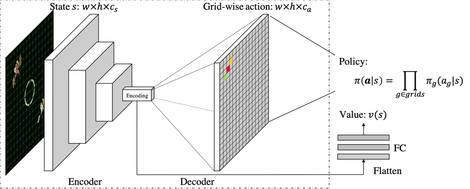
To bring a solution to the MARL problem we define a well known architecture in deep learning : an encoder-decoder ⏳ .

We will present this architecture layer by layer in a rather static way. Then we will see how it works and the different algorithms it uses to train the agents.

Notation

• State grid : $s \in \mathbb{R}^{w \times h \times c_{s}}$.
• State channels : $c_{s} \in \mathbb{N}^{*} $.
• Action map : $a \in \mathbb{R}^{w \times h \times c_{a}}$.
• Action map channels : $c_{a} \in \mathbb{N}^{*} $.
• Joint action space : $U=U_{1} \times U_{2} \times \cdots \times U_{n_{t}}$ with ${{1,2, \cdots, n_{t}}}$ is the set of agents.
• Possible joint action : $u \in U$.
• Possible action for agent $i$ : $u_{i} \in U_{i}$.
• Probability of taking each action for the agent located in $(i,j)$ in the action map $a$ : $a_{i,j} \in [0,1]^{c_{a}} = P(u|s)_{i,j}$ (probability vector).

Input layer

• Input tensor : The state grid $s \in \mathbb{R}^{w \times h \times c_{s}}$ where $w$ is the width of the grid, $h$ is the height and $c_{s}$ the feature number. We can see this tensor as a stack of $c_s$ feature maps on our agents and our environment.

  Let’s take an example : Let’s imagine that we want to train a set of agents to destroy the ennemy bases.

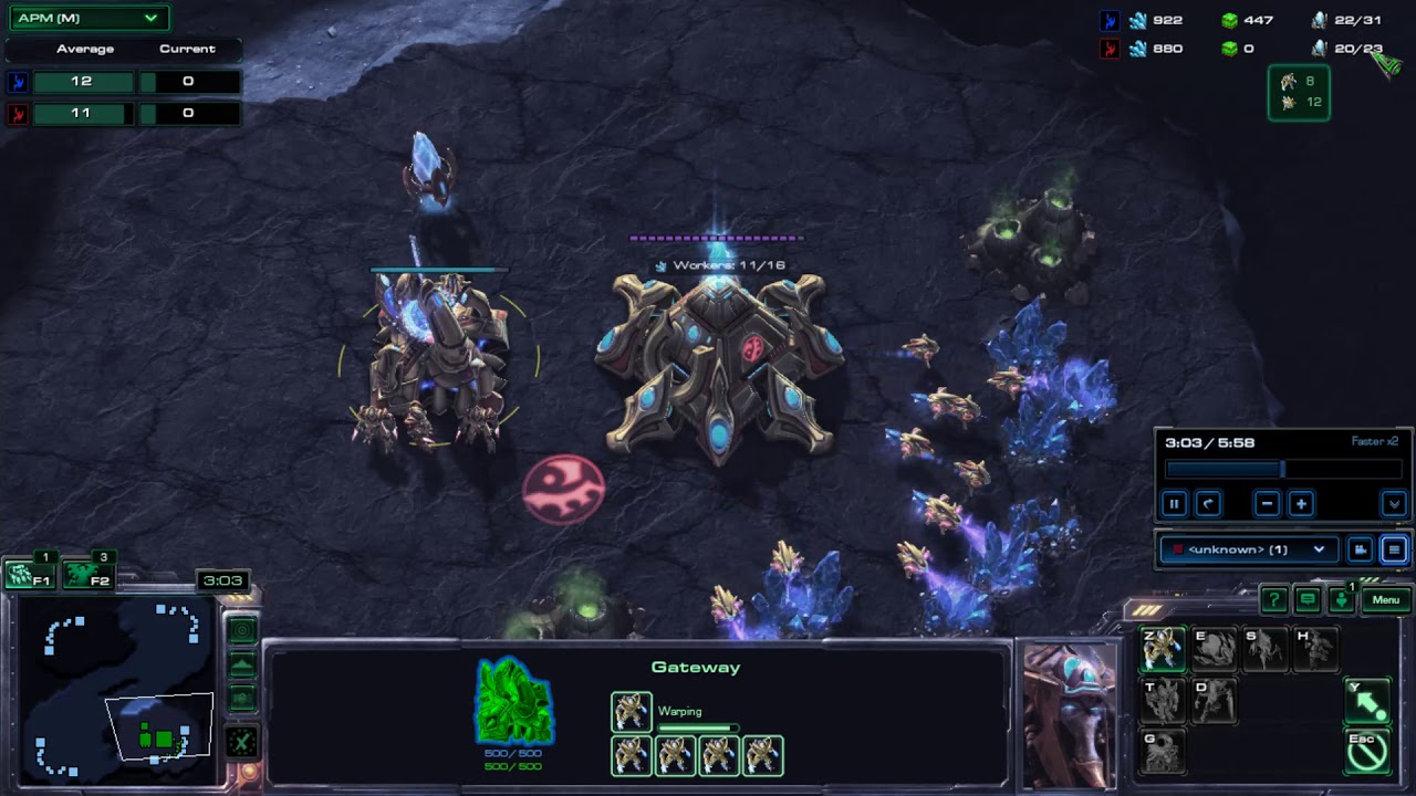
Our architecture can’t take that image. We have to find a way to encode the relevant information of the environment and the agents in the form of a set of grids (a tensor).

To describe our image we can give a set of grids as the following image:

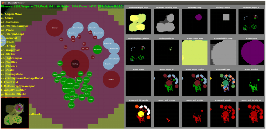
Each feature map (to the right of the image) represents relevant information about the environment and the local environment of our agents. Some information present on the initial image is deliberately hidden because it is useless.

For example the feature map on the first line in the 4th position represents the player’s camera. This is a more than relevant information!

This way we can create full feature tensors that represent the current state of our agents in the environment. We can then give this tensor to our network.

Encoder block :

• Convolutional encoder : The state $s$ (our feature tensor, a stack of feature maps) is fed to a convolutional network. This will create a latent representation of our state $s$ (our feature tensor). This representation is a good summary our state . “It also naturally handles agent collaboration, because the stacked convolutional layers can provide sufficiently large receptive field for the agents to communicate. The GridNet also enables fast parallel exploration, because experiences from one agent are immediately transferred to others through the shared convolutional parameters." The latent vector resulting from these successive convolutions (called encoding on the image) is a good summary of the state $s$, indeed it takes into account the situation of each agent as well as the collective dynamics.

Decoder block :

• Convolutional Decoder : The embedding $s_{encoded}$ of our state $s$ is fed into a Deconvolutional network. This will decod the latent representation of our state $s$. I remind you that this state concentrates the information of each agent as well as their collective dynamics. We want to decode this latent vector and give it a form of action grid (we will see this in the next paragraph). To do this we proceed to deconvolution and upsampling operations to increase the dimension of this vector. These upsampling operations result in an action grid $a \in \mathbb{R}^{w \times h \times c_{a}}$ where $c_{a}$ is the action number. For example if our agents are in a square zone of 20 length and that each agent has 4 actions then the action grid will have the following dimension $(20 \times 20 \times 4)$.

Output tensor : action map

• Let’s call back :

  Probability of taking each action for the agent located in $(i,j)$ in the action map $a$ : $a_{i,j} \in [0,1]^{c_{a}} = P(u|s)_{i,j}$ (probability vector).

$$a_{i,j} = P(u|s)_{i,j} = \left[\begin{array}{c}P(u^{1}|s), \ P(u^{2}|s), \ … ,\ P(u^{c_{a}}|s)\end{array}\right]_{i,j}$$

To simply illustrate the situation : Imagine that our agents have the same possible actions : $$ \forall i \in {1,…,n_{t}}, U_{i} = \left[\begin{array}{c}moveUp, \ moveDown, \ moveLeft, \ moveRight, \ shoot)\end{array}\right]$$ then for the agent located in $(i,j)$ in the action map $a$ we have : $$a_{i,j} = P(u|s)_{i,j} = \left[\begin{array}{c}P(moveUp|s), \ P(moveDown|s), \ P(moveLeft|s), \ P(moveRight|s),\ P(shoot|s)\end{array}\right]_{i,j}$$

Critic block

As you can see, our architecture has another element. Our network is divided in two : the encoder-decoder and what we will call the critic block. Once the information is encoded, we will extract via a fully connected layer the value function. We will explain what this function is in the next part which will deal with the optimization of this network.

From now on, our architecture is well defined ! The question that comes from now on is : How to optimize our network to answer the MARL problem? With the policy gradient !

Network optimisation

A few obvious facts

Let’s summarize what we just said with this little diagram !

As you have just seen, this diagram adds extra information ! What I called ‘critical-output-value’ and also the ‘policy optimisation’.

Our architecture has 2 outputs : The action grid $a$ and the output value $v$. To optimize our network we must therefore minimize a loss function.

The optimization of this function corresponds to the last step of our diagram !

The question that comes naturally now is the choice of that loss function.

Policy optimisation and Actor-critic

The purpose of our architecture is to give us for a state the best possible action (to maximize the reward). Our architecture therefore serves to optimize what we call policy $\pi$.

The policy is a function that gives us the probability of making an action $a$ knowing that we are in a certain state $s$. We want to optimize this policy so that our agent does the best sequence of actions (i.e. the sequence of actions that maximizes the reward).

In more mathematical terms, in that RL problem one seeks to optimize policy by maximize the following quantity :

$$\mathbb E_{\pi}\left[G_{t} \mid S_{t}=s\right]$$ $$=\mathbb{E}_{\pi}\left[\sum_{k=0}^{\infty} \gamma^{k} R_{t+k+1} \mid S_{t}=s\right]$$

Where $\gamma \in [0,1]$ is the discount-factor, $R_{t}$ is the reward at step $t$ and $S_{t}$ the state at step $t$.

We have to find the best policy $\pi$ in order to maximize the future rewards.

Let’s cut the suspens ! This is our loss function $J$ :

$$J(\theta)=\mathbb E_{s,u}\left[\log \pi_{\theta}\left(u \mid s\right){A}_{\pi}(s,u)\right]$$

Let’s explain the different components of this formula :

• $\log \pi_{\theta}\left(u \mid s\right)$ : it’s the output of the actor-network. We take the log probability of that output (i.e the log -probability to take action $u$ knowing we are in state s).

• $A_{\pi}(s, {a})=r(s,a)+v\left(s^{\prime}\right)-v(s)$ is what we called the Advantage-function. Where $\mathbf r$ is the reward function, $\mathbf v$ the value function (output of the critic-network), $\mathbf s$ is the current state and $\mathbf s'$ is the next state (i.e the state resulting of the The state resulting from action $\mathbf u$).

What is the intuition behind this function? Let’s take inspiration from Adil Zouitine’s paper note :

• If the avantage estimate was positive meaning that the action took by the agent in the sample trajectory resulted in better than average return we’ll do is increase the probability of selecting this action in the future when we encouter the same state (gradient is “positive”, increase these action probability). In mathematical terms :

$$A_{\pi}(s, a)=r(s, a)+v\left(s^{\prime}\right)-v(s) > 0 \implies sign(\nabla_{\theta} J(\theta)) = sign(\nabla_{\theta} \log \pi_{\theta}({u} \mid s))$$ $\rightarrow update(\theta) \ to \ increase \ \pi_{\theta}(a|s) $

If the avantage estimate was negative meaning the action took by the agent in the sample trajectory resulted in worst than average return we’ll do is decrease the probability of selecting this action in the future when we encouter the same state (gradient is “negative”, decrease these action probability)

$$A_{\pi}(s, a)=r(s, a)+v\left(s^{\prime}\right)-v(s) \leq 0 \implies sign(\nabla_{\theta} J(\theta)) = -sign(\nabla_{\theta} \log \pi_{\theta}({u} \mid s))$$ $\rightarrow update(\theta) \ to \ decrease \ \pi_{\theta}(u|s) $

For a more detailed explanation of the algorithm, here are some references :

• The reference book in RL presenting the actor-critics algorithm :

  • Reinforcement Learning : An Introduction page 257

• For the bravest and most mathematically minded among you, a blog post explaining in detail several policy gradient algorithms :

  • Lil’Log : Policy gradient Algorithms

Training iteration

In the previous section we have seen how to optimize an actor-critic algorithm.

The following diagram summarizes the entire process of optimizing our network.

Pseudo-code

Actor-Critic architecture implementation in pytorch

Here is an example of Gridnet implementation. This implementation is only a trivial and probably incorrect example. This example is just here to give an idea of the implementation.

• Encoder :

  

  class ConvBlock(nn.Module):
      # Convolution block : Conv + pooling
  
      def __init__(self, in_channels, out_channels):
          super(ConvBlock, self).__init__()
          self.conv1 = nn.Conv2d(
              in_channels=in_channels,
              out_channels=out_channels,
              kernel_size=3,
              padding=1,
              stride=1,
          )
          self.relu = torch.nn.ReLU()
          self.conv2 = nn.Conv2d(
              in_channels=out_channels,
              out_channels=out_channels,
              kernel_size=3,
              padding=1,
          )
          self.pool = torch.nn.MaxPool2d(kernel_size=2, stride=2)
  
      def forward(self, x):
  
          x = self.conv1(x)
          x = self.relu(x)
          x = self.conv2(x)
          x = self.relu(x)
          x = self.pool(x)
  
          return x
  
  class Encoder(nn.Module):
      def __init__(self, c_s, c_encodded):
          super(Encoder, self).__init__()
  
          self.block1 = ConvBlock(in_channels=c_s, out_channels=64)
          self.block2 = ConvBlock(in_channels=64, out_channels=128)
          self.block3 = ConvBlock(in_channels=128, out_channels=256)
          self.block4 = ConvBlock(in_channels=256, out_channels=c_encodded)
  
      def forward(self, x):
  
          for block in [self.block1, self.block2, self.block3, self.block4]:
              x = block(x)
  
          self.encodding = x
  
          return x
  

• Decoder :

  

  class DeconvBlock(nn.Module):
      # DeConvolution block : Conv + pooling
  
      def __init__(self, in_channels, out_channels):
          super(DeconvBlock, self).__init__()
  
          self.deconv = torch.nn.ConvTranspose2d(
              in_channels=in_channels, out_channels=in_channels, kernel_size=2, stride=2
          )
          self.conv1 = nn.Conv2d(
              in_channels=in_channels,
              out_channels=out_channels,
              kernel_size=3,
              padding=1,
              stride=1,
          )
          self.relu = torch.nn.ReLU()
          self.conv2 = nn.Conv2d(
              in_channels=out_channels,
              out_channels=out_channels,
              kernel_size=3,
              padding=1,
          )
  
      def forward(self, x):
  
          x = self.deconv(x)
          x = self.relu(x)
          x = self.conv1(x)
          x = self.relu(x)
          x = self.conv2(x)
  
          return x
  
  
  class Decoder(nn.Module):
      def __init__(self, c_encodded, c_a):
          super(Decoder, self).__init__()
  
          self.block1 = DeconvBlock(in_channels=c_encodded, out_channels=c_encodded // 2)
          self.block2 = DeconvBlock(
              in_channels=c_encodded // 2, out_channels=c_encodded // 4
          )
          self.block3 = DeconvBlock(
              in_channels=c_encodded // 4, out_channels=c_encodded // 8
          )
          self.block4 = DeconvBlock(in_channels=c_encodded // 8, out_channels=c_a)
  
      def forward(self, x):
  
          for block in [self.block1, self.block2, self.block3, self.block4]:
              x = block(x)
  
          return x
  
  

• Auto-encoder :

  

  
  class AutoEncoder(nn.Module):
      # Actor
      def __init__(self, c_s, c_encodded, c_a):
          super(AutoEncoder, self).__init__()
          self.encoder = Encoder(c_s=c_s, c_encodded=c_encodded)
          self.decoder = Decoder(c_encodded=c_encodded, c_a=c_a)
  
      def forward(self, x):
          embedding = self.encoder(x)
          actions_logit = self.decoder(embedding)
  
          return embedding, actions_logit
  

• Value function head :

  

  class ValueFunctionHead(nn.Module):
      # Critic
      def __init__(self, c_encodded, w_encodded, h_encodded):
          super(ValueFunctionHead, self).__init__()
  
          size_encodded = w_encodded * h_encodded * c_encodded)
  
          self.head = nn.Sequential(
              *[
                  nn.Flatten(),
                  nn.Linear(in_features=size_encodded, out_features=128),
                  torch.nn.ReLU(),
                  nn.Linear(in_features=128, out_features=1),
              ]
          )
  
      def forward(self, x):
          return self.head(x)
  

• Architecture :

  class GridNet(nn.Module):
      def __init__(self, c_s, c_encodded, w_encodded, h_encodded, c_a):
          super(GridNet, self).__init__()
  
          size_embedded = c_encodded, w_encodded, h_encodded
          self.auto_encoder = AutoEncoder(c_s=c_s, c_encodded=c_encodded, c_a=c_a)
          self.value_function_head = ValueFunctionHead(
              c_encodded=c_encodded, w_encodded=w_encodded, h_encodded=h_encodded
          )
          self.softmax = torch.nn.Softmax(dim=1)
  
      def forward(self, x):
          embedding, actions_logit = self.auto_encoder(x)
          action_map = self.softmax(actions_logit)
          value_function = self.value_function_head(embedding)
  
          return {"Actor": action_map, "Critic": value_function}
  

Result